Continuous Random Variables

5 concepts

In this chapter

This chapter extends chapter 1's distinction from data already collected to random variables whose value isn't known yet: when the possible outcomes fill an interval rather than a countable list, probability has to be measured as area under a curve, not read off a table of outcomes. From that one idea it builds two of the standard continuous models — the uniform distribution's flat density over an interval, and the exponential distribution's model of a random wait, including the memoryless property that makes it distinctive.

Outcomes That Fill an Interval, Not a List

Definition

A random variable is continuous when its possible outcomes fill an interval on the real line rather than forming a separate, countable list — the same discrete/continuous test chapter 1 applied to data, applied here to an outcome not yet observed.

The test

Ask whether a value strictly between two others can occur, in principle. A count of events, successes, or items cannot; a measured time, length, or amount can, no matter how finely you look.

Example

A hypothetical customer's decision time at a vending machine can fall anywhere on a stretch of seconds; the number of items the same customer buys cannot fall between 2 and 3. The first is continuous; the second is discrete.

The trap

"A stopwatch only displays two decimal places, so the time itself must be discrete." The display rounds a continuous quantity; it doesn't change what's being measured — the true elapsed time can still, in principle, land anywhere in between. "A continuous variable can still be listed, just with a lot of values." Between any two continuous values sits another one, endlessly — there is no next value to list, which is exactly why the list-based probability of earlier chapters needs replacing with area.

Probability as the Area Under a Density Curve

Definition

A probability density function $f(x)$ describes a continuous random variable so that probability is the area beneath its curve over an interval, not the curve's height at a single point.

The test

For any interval, probability is area — base times height for a flat stretch, more generally the region under the curve — and the total area over every possible value is exactly 1. For any single exact value the interval has zero width, so the area, and the probability, is zero: $P(X=x)=0$ .

Example

A hypothetical dial spinner lands anywhere on the interval from 0 to 10 with a flat density of 0.1. The probability it lands between 2 and 6 is the rectangle's area, $4 \times 0.1 = 0.4$ ; the probability it lands on exactly $x=6$ is $0 \times 0.1 = 0$ .

A hypothetical continuous density curve: the shaded region between two points is a probability, while a single point, having zero width, encloses zero area and therefore zero probability.drawn by figures/fig-density-area.py

The trap

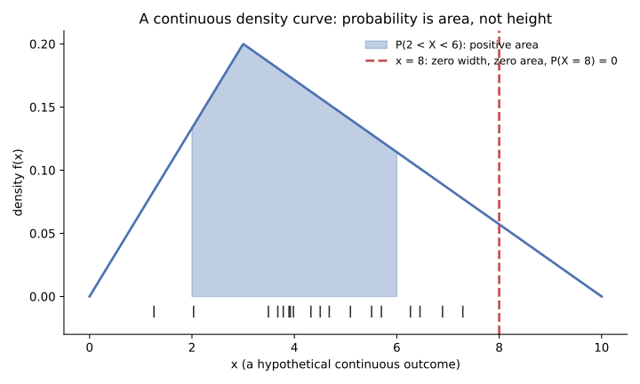
"The probability at exactly $x$ is the height of the curve, $f(x)$ ." $f(x)$ is a density, not a probability — it only becomes a probability once multiplied by a width, and a single point's width is zero. "Since $P(X=x)=0$ for every $x$ , no value is actually possible." Some value always occurs; it is only that no single value carries positive probability on its own — only intervals do.

The Uniform Distribution: A Flat Density Over an Interval

Definition

A continuous random variable $X$ is uniformly distributed, written $X \sim U(a,b)$ , when its density is the constant $\displaystyle f(x) = \frac{1}{b-a}$ for every $x$ between $a$ and $b$ .

The test

Confirm the density is flat across a fixed interval $[a,b]$ . If so, the probability of any sub-interval $(c,d)$ is area: width times the constant height, $\displaystyle (d-c)\cdot\frac{1}{b-a}$ , regardless of where in $[a,b]$ that sub-interval sits. Its centre and spread follow from the endpoints alone: $\displaystyle \mu = \frac{a+b}{2}$ and $\sigma = \sqrt{\frac{(b-a)^2}{12}}$ .

Example

A hypothetical campus shuttle arrives equally likely at any minute from 0 to 24 past the hour: $X \sim U(0,24)$ , so $f(x) = \frac{1}{24}$ on that interval.

Worked example

Confirm the density. $X \sim U(0,24)$ , so $f(x) = \frac{1}{24}$ for every $x$ in $[0,24]$ .
Find the interval's width. For $P(5<X<11)$ , the width is $11-5=6$ .
Multiply width by height. $\displaystyle P(5<X<11) = 6 \times \frac{1}{24} = 0.25$ .

Common slips: using the interval's width alone without multiplying by $\displaystyle \frac{1}{b-a}$ ; subtracting the endpoints in the wrong order.

The trap

"The probability of an interval is just its width." Width alone omits the height: a 6-minute window is $6 \times \frac{1}{24}$ , not 6. "'Uniform' means every exact value is equally likely, the way a die's six faces are." Density is constant, but every single value still has probability zero, exactly as the previous section established — "uniform" describes the flat curve, not equally likely points.

The Exponential Distribution: Modeling a Random Wait

Definition

The exponential distribution, $X \sim \text{Exp}(m)$ , models the waiting time until a random event, with density $f(x) = me^{-mx}$ for $x \ge 0$ , where the rate parameter $m$ — written $\lambda$ almost everywhere outside this book — is the reciprocal of the mean wait, $m=\frac{1}{\mu}$ . Its standard deviation equals its mean.

The test

Ask whether the quantity is a wait until something happens, with short waits more common than long ones. The 's density is flat; the exponential density is tallest at $x=0$ and shrinks as $x$ grows, with cumulative probability $P(X<x) = 1-e^{-mx}$ .

Example

Support tickets arrive with a mean wait of 5 minutes until the next one (hypothetical): $X \sim \text{Exp}(0.2)$ , since $\displaystyle m=\frac{1}{5}=0.2$ .

Worked example

Find the rate parameter. Mean wait $\mu=5$ minutes, so $\displaystyle m=\frac{1}{\mu}=\frac{1}{5}=0.2$ .
Apply the cumulative distribution function (CDF (cumulative distribution function)). $P(X<x) = 1-e^{-mx}$ .
Substitute and compute. $\displaystyle P(X<3) = 1-e^{-0.2\times3} = 1-e^{-0.6} \approx 1-0.5488 = 0.4512$ .

Common slips: substituting the mean $\mu$ for $m$ instead of its reciprocal; dropping the negative sign in the exponent.

Expanded

Checking this in software, without getting a wrong answer quietly. Tools disagree about which number you hand them. R asks for the rate directly, so pexp(3, rate = 0.2) reproduces the 0.4512 above. Python's SciPy asks for the scale, which is the reciprocal of the rate: the correct call is expon.cdf(3, scale = 1/0.2), that is scale = 5. Writing expon.cdf(3, 0.2) looks right and is not — the second positional argument is a shift, not a rate, so the call succeeds and returns a different number with no error raised. This is the failure worth naming: a tool that disagrees loudly costs a minute, and one that disagrees silently costs a learner their confidence in arithmetic that was correct all along. When a result here and a result on screen differ, check which parameter the function wants before you doubt the method.

Two continuous density shapes compared: the uniform distribution's flat rectangle (left, shading the same 5-to-11-minute window worked out in the text) against the exponential distribution's front-loaded, decaying curve (right, shading the same under-3-minute wait worked out in the text).drawn by figures/fig-uniform-vs-exponential.py

The trap

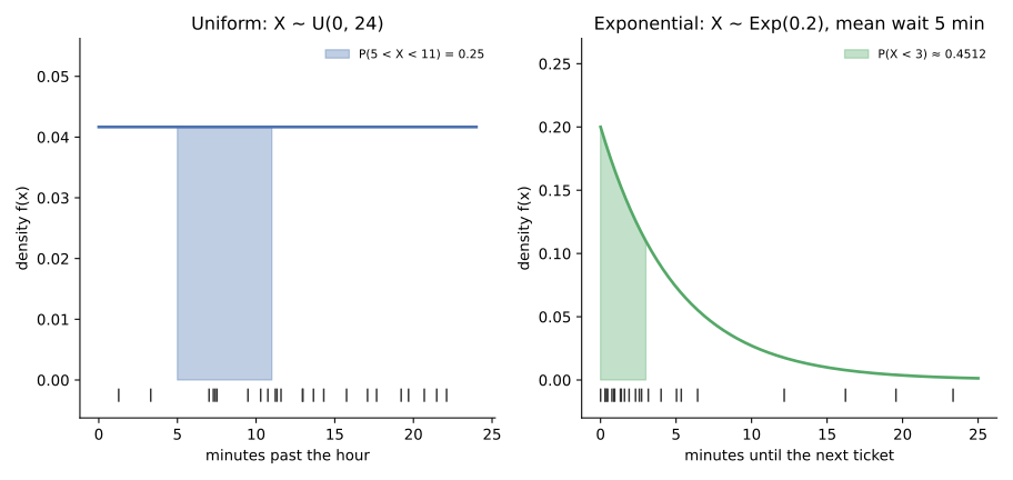
"The rate parameter is the average wait, so $m=0.2$ means a typical wait of 0.2 minutes." A rate counts events per unit of time, and the mean wait is its reciprocal: $\mu = \frac{1}{m} = 5$ minutes. A bigger $m$ therefore means events arrive more often and waits get shorter, not longer. "One fixed rate means waits arrive at evenly spaced intervals." The rate describes the average over many waits, not the pattern of any one wait — individual wait times vary randomly and are usually short, occasionally long.

Expanded

The exponential distribution has a close discrete relative. If the wait between successive events is exponential with mean $\mu$ , the count of such events in one fixed unit of time follows a distribution built for counting events in an interval, with average rate $\displaystyle \lambda=\frac{1}{\mu}$ — the same underlying random process, described once as a continuous wait between events and once as a discrete count of events. That discrete count is a separate concept, covered where discrete random variables are built up.

The Memoryless Property: Why the Wait Forgets the Past

Definition

The 's memoryless property states that surviving to time $r$ changes nothing about the remaining wait: $P(X>r+t \mid X>r) = P(X>t)$ for every $r,t \ge 0$ .

The test

Compare the conditional probability of surviving $t$ more units, given survival to $r$ already, against the probability a fresh draw survives $t$ units from zero. For the exponential distribution the two are always algebraically equal; for most other distributions they are not.

Example

A hypothetical component's lifetime has a mean of 8 years, so its rate parameter is $\displaystyle m=\frac{1}{8}=0.125$ . Having already run 3 years, the probability it lasts 5 more years equals the probability a brand-new component lasts 5 years: $\displaystyle P(X>5)=e^{-0.125 \times 5}=e^{-0.625}\approx 0.5353$ .

An exponential density (solid) and the same curve shifted to start at an elapsed time of 3 years (dashed): the shifted tail exactly overlays a fresh curve from zero, the visual signature of the memoryless property.drawn by figures/fig-memoryless.py

The trap

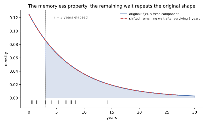
"Memoryless means the component doesn't age." True only in the narrow sense that the model has no built-in wear; it does not mean nothing changes physically, only that past survival carries no probabilistic information about the remaining wait. "Having survived unusually long, it must be 'due' to fail soon." The gambler's-fallacy reading; the property says the exact opposite — elapsed time never raises or lowers the remaining-wait probability.

Putting Continuous Probability to WorkSynthesis

One more hypothetical: an emergency room's wait time. Before it's measured, the wait is a random variable — it can land anywhere on a stretch of minutes, not a fixed list — so its probabilities are , not a table of chances, and its probability of any single exact minute is zero however likely that stretch feels.

If every wait length in a range were equally plausible, a would fit: constant density, equal-width windows carrying equal probability wherever they fall. Real waits usually don't behave that way — short waits are typically more common than long ones — which pulls in the instead, its density tallest at zero and falling as the wait grows, set by a single parameter that is the reciprocal of the mean wait.

The exponential model carries one further, sharper claim, its : a patient who has already waited 20 minutes is no more or less likely to wait 10 more than one just walking in — "waiting a long time already" is not, on its own, evidence a wait is nearly over.

Sources

1 OpenStax Introductory Statistics §5.1: Continuous Probability Functions — source
2 OpenStax Introductory Statistics §5.2: The Uniform Distribution — source
3 OpenStax Introductory Statistics §5.3: The Exponential Distribution — source
4 NIST/SEMATECH e-Handbook §1.3.6.6.2: Uniform Distribution (mean (A+B)/2, standard deviation sqrt((B-A)^2/12)) — source
5 SciPy scipy.stats.expon documentation — the exponential is parameterized by the rate lambda, supplied as scale = 1/lambda — source