Discrete Random Variables

6 concepts

In this chapter

This chapter turns a random process into a number you can compute with: a discrete , its , and the two summary numbers, and , that describe it without listing every outcome. It closes with the single most common shape a discrete random variable takes in practice, the , and the for its own mean and standard deviation.

What a Random Variable Is

Definition

A random variable assigns a number to the outcome of a random process, before the outcome is known; it is discrete when its possible values can be counted and listed, with real gaps between them.

The test

Ask two things: does it assign a number to an outcome not yet known? If so, it is a random variable. Then apply the same counting-versus-measuring test chapter 1 used for : can a value fall strictly between two consecutive possible values? If no, it is discrete.

Example

A food truck owner tracks the number of food-allergy special orders in a randomly chosen lunch hour (hypothetical). The count can only be 0, 1, 2, 3, and so on, with nothing valid between 1 and 2, so it is a discrete random variable.

The trap

"Writing 'X = 3' and saying 'there's a 30% chance' are the same kind of statement." They are not: $X$ names a value the variable could take, while $P(X=3)$ names how likely that value is — a random variable and its probability are different things. "A discrete random variable's values always have to be consecutive whole numbers starting at 0." Discreteness only requires listable values with real gaps between them; negative numbers, skipped values, or uneven spacing are still discrete.

Building a Valid Probability Distribution

Definition

A discrete random variable's probability mass function, or PMF (probability mass function), pairs every value it can take with the probability of that value.

The test

A table is a valid PMF (probability mass function) only when both hold: every probability is between 0 and 1 inclusive, and all the probabilities sum to exactly 1. Passing only one rule is not enough.

Example

The food truck owner drafts a table for 0, 1, 2, or 3 special orders per lunch hour: probabilities 0.35, 0.30, 0.25, 0.10. Each is between 0 and 1, and they sum to 1, so the table is a valid PMF (probability mass function).

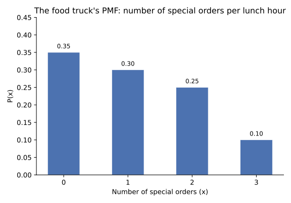
The food truck's probability mass function: four bars, one per possible number of special orders, with heights that sum to 1.drawn by figures/fig-pmf-bar-chart.py

The trap

"As long as every number is a legitimate probability, the table counts as valid." Not enough alone: a table of 0.35, 0.30, 0.25, 0.20 has four legal-looking numbers that sum to 1.10, claiming more than certainty across outcomes meant to cover every possibility. "A probability distribution has to spread probability equally across every value, or it isn't really random." Nothing requires equal probabilities; a distribution favoring one value heavily is exactly as valid as an even one, provided both rules above hold.

Expected Value: The Long-Run Average

Definition

The expected value, written $\mu$ , is a discrete random variable's long-run average outcome over many repetitions.

The test

Multiply each possible value by its own probability, then add the products: $\mu = \sum x \cdot P(x)$ . This describes where outcomes center over many repetitions, not what happens on any single trial.

Example

For the food truck's table, computing $\mu$ from 0.35, 0.30, 0.25, 0.10 gives a long-run average that is not one of 0, 1, 2, or 3 — shown step by step below.

Worked example

List each value and its probability. From the table: $x = 0, 1, 2, 3$ with $P(x) = 0.35, 0.30, 0.25, 0.10$ .
Multiply each value by its probability. $0(0.35)=0$ ; $1(0.30)=0.30$ ; $2(0.25)=0.50$ ; $3(0.10)=0.30$ .
Add the products. $\mu = 0 + 0.30 + 0.50 + 0.30 = 1.10$ special orders.

Common slips: averaging the four $x$ values without weighting by probability at all; dividing the summed products by the number of outcomes (4), which double-counts weighting already done in step 2.

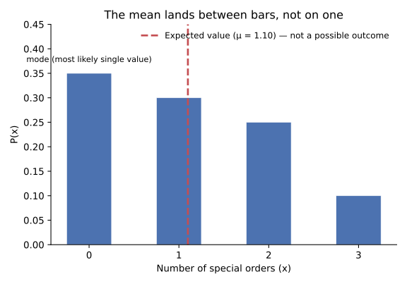
The same distribution with its expected value marked: the dashed line lands between two bars, not on one, because the mean need not be a value the random variable can actually take.drawn by figures/fig-expected-value-marked.py

The trap

"The expected value is the value you'd most expect on any one trial — the most likely outcome." That quantity is the mode, and often disagrees with $\mu$ : here 0 is the single most likely count, at probability 0.35, yet $\mu = 1.10$ . "Since it's an average, the expected value has to be one of the values the variable can take." It does not: an average of whole numbers is rarely a whole number itself, the same way a class's average sibling count can be 1.8 with no student actually having 1.8 siblings.

Standard Deviation: How Far Outcomes Stray

Definition

The standard deviation, written $\sigma$ , measures how far a random variable's outcomes typically spread from its $\mu$ .

The test

Square each value's distance from $\mu$ so distances above and below do not cancel, weight each by its probability, sum, then take the square root: $\sigma = \sqrt{\sum (x-\mu)^2 \cdot P(x)}$ .

Example

For the food truck's table, $\mu = 1.10$ ; weighting each squared distance from 1.10 by its probability and summing gives 0.99, so $\sigma = \sqrt{0.99} \approx 0.99$ special orders.

The trap

"A standard deviation of 0 means the calculation went wrong, since a random variable is supposed to vary." It is not an error: $\sigma = 0$ correctly describes a random variable that always takes the same single value, with no variation at all. "Standard deviation and expected value are basically measuring the same thing." They answer different questions: $\mu$ asks where outcomes center; $\sigma$ asks how far they typically wander from there, and two random variables can share one while differing sharply in the other.

The Binomial Distribution and When It Applies

Definition

A binomial random variable counts the number of successes across $n$ independent trials, each with the same two possible outcomes and the same probability of success $p$ ; written $X \sim B(n,p)$ .

The test

Check all three together: a fixed number of trials $n$ ; exactly two outcomes per trial, success (probability $p$ ) and failure (probability $q = 1-p$ ); and trials that are independent, with $p$ unchanged from one trial to the next.

Example

A basketball player makes 70% of free throws, each attempt treated as independent of the others (hypothetical), and attempts 8. "Number made" is binomial with $n=8$ , $p=0.70$ . What is the probability she makes exactly 6?

Worked example

Confirm the conditions and identify $n$ , $p$ , $x$ . Fixed trials, two outcomes, and independent, constant probability all hold; here $n=8$ , $p=0.70$ , $q=0.30$ , target $x=6$ .
Count the arrangements. $\displaystyle \binom{n}{x} = \binom{8}{6} = 28$ — the number of orders 6 makes and 2 misses could occur in across 8 attempts.
Compute one arrangement's probability. $\displaystyle p^{x}q^{n-x} = 0.70^{6} \times 0.30^{2} \approx 0.1176 \times 0.09 \approx 0.01059$ .
Multiply. $\displaystyle P(6) = 28 \times 0.01059 \approx 0.2965$ — about a 30% chance of exactly 6 makes.

Common slips: leaving out $\displaystyle \binom{n}{x}$ , which gives the probability of one specific order of makes and misses, not all of them; swapping the exponents, $p^{n-x}q^{x}$ , which computes the probability of $x$ misses instead of $x$ successes.

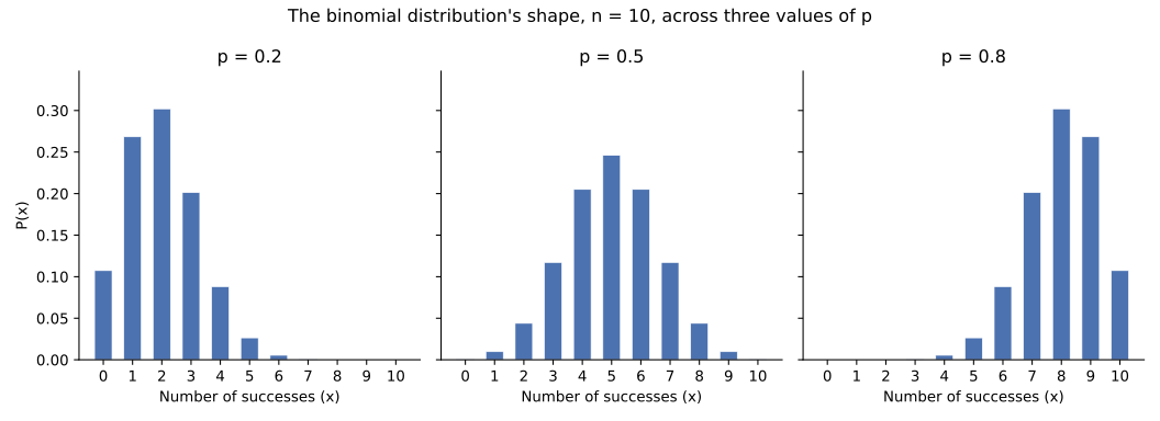
At fixed n = 10, the binomial distribution is right-skewed at p = 0.2, with a long tail toward larger success counts; symmetric at p = 0.5; and left-skewed at p = 0.8, with a long tail toward smaller success counts.drawn by figures/fig-binomial-shape.pyThis figure becomes interactive in the app.

The trap

"Any count of 'successes out of some tries' qualifies as binomial." Not if the tries affect each other: drawing 8 cards without replacement to count reds changes the probability on every draw, breaking independence — a different distribution applies there. "'At least' can be answered by computing the probability of exactly that one number." "At least 6" asks about a range, $x = 6, 7,$ and $8$ together, not the single value $P(6)$ alone.

Mean and Standard Deviation of a Binomial Random Variable

Definition

A binomial random variable's and simplify to $\mu = np$ and $\displaystyle \sigma = \sqrt{npq}$ , without needing the full probability table.

The test

Multiply $n$ by $p$ for the mean; multiply $n$ by $p$ by $q$ and take the square root for the standard deviation. Both hold for any valid $p$ , not only $p = 0.5$ .

Example

For the free-throw shooter, $n=8$ , $p=0.70$ , $q=0.30$ : $\mu = 8 \times 0.70 = 5.6$ expected makes; $\sigma = \sqrt{8 \times 0.70 \times 0.30} = \sqrt{1.68} \approx 1.30$ makes.

The trap

"The shortcut $\mu=np$ only works when $p=0.5$ ." It holds for every valid $p$ ; $p=0.5$ is simply the easiest case to check by hand, since success and failure are equally likely there. " $\mu=np$ always comes out to a whole number, matching an actual possible count." Here $\mu = 5.6$ , a value she can never actually make in one game of 8 attempts — the same "average need not be achievable" fact from applies to this shortcut too.

Seeing the Whole Distribution at OnceSynthesis

One last hypothetical: a call center where each incoming call is independently resolved on the first try with probability 0.6, and a supervisor tracks first-try resolutions out of 5 calls.

That count is a : a number attached to an outcome not yet observed, taking the listable values 0 through 5. Writing its means pairing each of those six values with a probability, valid only if every entry sits between 0 and 1 and all six sum to exactly 1. Every trial is independent with the same two outcomes and the same fixed probability, so the count is also binomial, $X \sim B(5, 0.6)$ , and its and both reduce to short expressions in $n$ and $p$ .

The , $\mu = np = 3$ , describes the long-run average across many five-call stretches, not a guarantee about this one; the , $\displaystyle \sigma = \sqrt{npq} \approx 1.10$ , describes how far a typical stretch strays from that average. Neither number promises what happens next; together they describe the shape of what tends to happen across many repetitions, seen once as a table and once as a formula.

Sources

1 OpenStax Introductory Statistics §4.1: Probability Distribution Function (PDF) for a Discrete Random Variable — source
2 OpenStax Introductory Statistics §4.2: Mean or Expected Value and Standard Deviation — source
3 OpenStax Introductory Statistics §4.3: Binomial Distribution — source
4 NIST/SEMATECH e-Handbook of Statistical Methods §1.3.6.6.18: Binomial Distribution (states the closed-form PMF and the mean np, SD √(np(1−p))) — source