Probability Topics

7 concepts

In this chapter

The first chapter asked how well a sample stands in for a population; this chapter turns to a different question — given everything that could happen, how likely is any one thing? It builds the vocabulary of , the operations that combine them (), and the difference between events that are and events that merely cannot overlap. It closes with two ways of reading probabilities off real data: and .

Sample Spaces, Outcomes, and Events

Definition

A sample space is the complete list of every outcome an experiment could produce; an event is any subset of that sample space — one outcome, several, or none — and its probability, written $P(A)$ , is a number from 0 to 1 measuring how likely it is.

The test

List every distinct outcome; that list is the sample space. An event is whichever subset of it you actually care about. When outcomes are equally likely, $P(A)$ is the count satisfying $A$ divided by the total count in the sample space.

Example

An 8-slice spinner, slices numbered 1 to 8, equally likely (hypothetical). The sample space is $S = \{1, 2, \ldots, 8\}$ . Event $A$ , "lands on an odd number," is $\{1, 3, 5, 7\}$ , so $P(A) = 4/8 = 0.5$ .

The trap

"An event is a single result — landing on 4." An outcome is one result; an event can gather several at once, like $A$ above. "Every dice total is equally likely, since nothing makes one more special." The 36 ordered pairs of two dice are equally likely, but their totals are not — only one pair sums to 2, while six different pairs sum to 7.

Combining Events: AND, OR, and Complement

Definition

For events $A$ and $B$ : $A$ AND $B$ is the outcomes in both; $A$ OR $B$ is the outcomes in either or both; the complement $A'$ is every outcome not in $A$ .

The test

AND narrows down to the overlap; OR gathers everything either event touches, counting the overlap once. Since every outcome is in $A$ or in $A'$ and never both, $P(A) + P(A') = 1$ always.

Example

Same spinner: $A$ = "odd" = $\{1,3,5,7\}$ , $B$ = "greater than 5" = $\{6,7,8\}$ . $A$ AND $B$ = $\{7\}$ ; $A$ OR $B$ = $\{1,3,5,6,7,8\}$ ; $A' = \{2,4,6,8\}$ , so $P(A') = 4/8 = 0.5 = 1 - P(A)$ .

The same scattered outcomes and two events, A and B, shaded three ways: A AND B (left), A OR B (middle), and the complement of A (right).drawn by figures/fig-events-and-or-complement.py

The trap

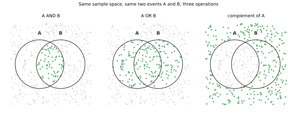
"'A or B' means one or the other, not both." Mathematical OR always includes both — unlike "coffee with cream or sugar," which usually rules both out. "The complement takes a fresh count, just like the original event did." $P(A')$ almost never needs recounting: $1 - P(A)$ is faster and exact.

Conditional Probability: What Changes Once You Know Something

Definition

Conditional probability $P(A|B)$ is the probability that $A$ happens given that $B$ is already known to have happened: $P(A|B) = P(A \text{ AND } B) / P(B)$ .

The test

Learning that $B$ happened shrinks the sample space down to just $B$ 's outcomes. Ask how many of those remaining outcomes are also in $A$ , out of $B$ 's total, not the original total.

Example

Same spinner: $A$ = "odd," $B$ = "greater than 5." $P(A \text{ AND } B) = 1/8$ (only 7) and $P(B) = 3/8$ , so $P(A|B) = (1/8)/(3/8) = 1/3$ — lower than the plain $P(A) = 4/8$ .

The trap

"P(A given B) and P(B given A) are the same number, just reordered." They shrink to different sample spaces — here $P(B|A) = 1/4$ , not $1/3$ . "Learning B happened can't change A's probability." It changes exactly when $B$ rules out some of $A$ 's favorable outcomes, as it does here.

Independent Events Are Not Mutually Exclusive Events

Definition

Events are independent when knowing one happened doesn't change the other's probability: $P(A|B) = P(A)$ . Events are mutually exclusive when they share no outcomes and can never both happen: $P(A \text{ AND } B) = 0$ .

The test

Check independence with $P(A \text{ AND } B) = P(A)P(B)$ ; check mutual exclusivity with $P(A \text{ AND } B) = 0$ . Unless a problem states otherwise, assume events are dependent and not mutually exclusive until you can show one.

Example

A fair coin flipped twice (hypothetical): "heads on flip 1" and "heads on flip 2" are independent — $\displaystyle P(\text{H2}|\text{H1}) = 0.5 = P(\text{H2})$ — and not mutually exclusive, since both can happen together.

The trap

"Independent just means mutually exclusive — the events have nothing to do with each other." For events that can each happen, they're opposites: mutually exclusive events are maximally dependent, since one ruling out the other is the strongest dependence there is. "After five heads in a row, a tails is due." The flips are independent — the coin has no memory, so flip 6 stays 0.5 regardless of history.

The Multiplication and Addition Rules

Definition

The multiplication rule finds $P(A \text{ AND } B)$ ; the addition rule finds $P(A \text{ OR } B)$ . Each has a general form and a simpler special case that only applies once independence or mutual exclusivity has actually been checked.

The test

Multiplication: $\displaystyle P(A \text{ AND } B) = P(A) \cdot P(B|A)$ in general, or $P(A) \cdot P(B)$ if independent. Addition: $\displaystyle P(A \text{ OR } B) = P(A) + P(B) - P(A \text{ AND } B)$ in general, or $P(A) + P(B)$ if mutually exclusive.

Example

A hypothetical hiring pipeline: 60% of applicants pass a math screen; 50% pass a writing screen; among those who pass math, 75% also pass writing. The worked steps below find both the probability of passing both and the probability of passing at least one.

Worked example

Name what's known. $P(M) = 0.6$ , $P(W) = 0.5$ , $P(W|M) = 0.75$ .
Check independence first. $P(W|M) = 0.75 \ne P(W) = 0.5$ , so $M$ and $W$ are dependent — the general multiplication rule is required, not the shortcut.
Apply the multiplication rule. $\displaystyle P(M \text{ AND } W) = P(M) \cdot P(W|M) = 0.6 \times 0.75 = 0.45$ .
Apply the addition rule. $\displaystyle P(M \text{ OR } W) = P(M) + P(W) - P(M \text{ AND } W) = 0.6 + 0.5 - 0.45 = 0.65$ .

Common slips: multiplying $P(A)$ by $P(B)$ without checking independence first; forgetting to subtract $P(A \text{ AND } B)$ in the addition rule, which double-counts everyone in both.

Case

In 1654 the gambler Chevalier de Méré asked why a bet he trusted kept losing: at least one ace in four rolls of one die paid off consistently, so he wagered on at least one double-ace in twenty-four rolls of two dice, scaling the roll count sixfold to match the sixfold-rarer double. The two bets are not proportional — the first wins with probability near 0.518, the second only about 0.491 — because repeated-roll probabilities compound rather than scale in a straight line. De Méré's puzzle reached Blaise Pascal, whose resulting correspondence with Pierre de Fermat is credited with founding the mathematical theory of probability.

The trap

"You can always just multiply P(A) and P(B) to get P(A and B)." Only when independent — otherwise $P(A) \cdot P(B|A)$ is required, as above, where $0.6 \times 0.5 = 0.3$ would have been wrong. "The addition rule is just P(A) + P(B)." That over-counts the overlap unless the events are mutually exclusive; subtracting $P(A \text{ AND } B)$ is what fixes it.

Reading a Contingency Table

Definition

A contingency table cross-tabulates two categorical variables in rows and columns, so row totals, column totals, and cell counts can be turned into marginal, joint, and conditional probabilities.

The test

A marginal probability divides a row or column total by the grand total. A joint probability divides one cell by the grand total. A conditional probability divides one cell by its own row or column total — the word "given" always shrinks the denominator.

Example

A hypothetical gym cross-tabulates 200 members by membership type (Standard/Premium) against weekly-class attendance (yes/no). The worked steps below read three probabilities straight from the table.

Worked example

Read the table. Premium-and-attends = 30; Premium total = 50; grand total = 200.
Marginal probability. $P(\text{Premium}) = 50/200 = 0.25$ .
Joint probability. $\displaystyle P(\text{Premium AND attends}) = 30/200 = 0.15$ .
Conditional probability. $\displaystyle P(\text{attends} \mid \text{Premium}) = 30/50 = 0.6$ — divide by the Premium row total, not the grand total.

Common slips: dividing a conditional probability by the grand total instead of the relevant row or column total; swapping $P(\text{attends}\mid\text{Premium})$ for $P(\text{Premium}\mid\text{attends})$ , which divides the same 30 by a different total.

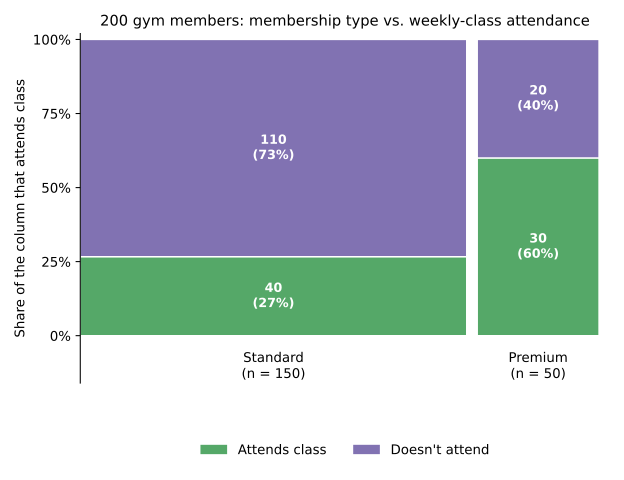
A mosaic of the 200-member gym example: column width shows how many members are Standard versus Premium, and the shaded height within each column shows what share of that group attends the weekly class.drawn by figures/fig-contingency-mosaic.py

The trap

"Every probability from the table divides by the grand total." Only marginal and joint probabilities do; a conditional probability divides by its row or column total instead. "P(attends given Premium) and P(Premium given attends) work out the same." They divide 30 by different totals — 50 versus the attends-column total of 70 — and rarely match.

Tree Diagrams and Venn Diagrams

Definition

A tree diagram shows a sequence of events as labeled branches, multiplied along each path; a Venn diagram shows events as overlapping regions in a box representing the sample space.

The test

On a tree diagram, multiply branch probabilities along one path; later branches can carry conditional probabilities that depend on the branch before them. On a Venn diagram, overlap is AND, combined area is OR, and outside a circle is that event's complement.

Example

A bag with 5 red and 3 blue marbles (hypothetical), drawn twice without replacement. The first branch pair is $5/8$ (red) and $3/8$ (blue); given red first, the second branch pair becomes $4/7$ and $3/7$ , so $\displaystyle P(\text{red, red}) = 5/8 \times 4/7$ .

A two-stage tree diagram for drawing two marbles without replacement from a bag of 5 red and 3 blue: branch probabilities change on the second draw because the first marble is not returned.drawn by figures/fig-tree-diagram.py

The trap

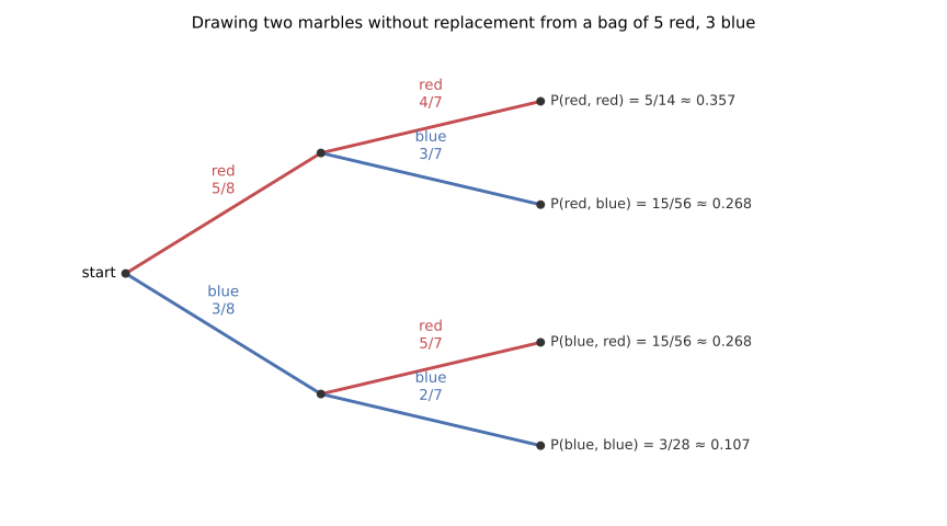
"You add branch probabilities along a path instead of multiplying." Multiplying applies the multiplication rule one branch at a time; adding belongs to combining separate paths, not one path's own steps. "A Venn diagram's circle sizes must match the real probabilities." Venn diagrams are schematic — a circle's drawn size carries no promise about its actual probability unless the diagram explicitly says so.

From Sample Space to Everyday OddsSynthesis

One last hypothetical ties the chapter together: a small clinic tracks 500 patients by test result (positive or negative) and whether they actually have a rare condition — a waiting to happen. The clinic's is all 500 patients; "tests positive" and "has the condition" are each an , and asking for one given the other is , not the plain marginal rate. The two events are not — a real test's result depends on the true condition — nor are they mutually exclusive, since both can hold at once. Finding "tests positive and has the condition" is the ; finding "tests positive or has the condition" is the addition rule. A can lay out condition-then-test as two levels of branches, multiplied along each path, while a Venn diagram can show the same relationship as two overlapping circles. None of these seven ideas is optional scaffolding: together they are the difference between reading a positive test as proof of the condition and reading it correctly, as evidence that shifts a probability without pinning it at 0 or 1.

Sources

1 OpenStax Introductory Statistics §3.1: Terminology — source
2 OpenStax Introductory Statistics §3.2: Independent and Mutually Exclusive Events — source
3 OpenStax Introductory Statistics §3.3: Two Basic Rules of Probability — source
4 OpenStax Introductory Statistics §3.4: Contingency Tables — source
5 OpenStax Introductory Statistics §3.5: Tree and Venn Diagrams — source
6 cut-the-knot.org: Chevalier de Méré's Problem — source
7 MacTutor History of Mathematics (Univ. of St Andrews): Pierre de Fermat — source