Sampling and Data

6 concepts

In this chapter

This chapter gives you the vocabulary and judgment for reading any sample-based claim critically: the relationship itself, how a sample goes bad even at a large size, and how to tell ordinary chance variation from a real problem. It closes with two further distinctions used on every dataset from here on: data, then, within quantitative data, data.

Why We Study Samples Instead of Everyone

Definition

A population is the entire group you want to know something about; a sample is the subset of it you actually examine.

The test

Ask which group the question is really about — the population — then check how much of it you measured. Full measurement is rare: it's usually too slow or costly, and sometimes destructive, as when a factory tests lightbulbs to failure.

Example

A university with 40,000 students wants to know dining-hall satisfaction (hypothetical). Surveying all 40,000 would be exact but slow and costly, so it surveys 300 instead: the population is all 40,000; the sample is the 300 asked.

The trap

"A bigger population needs a proportionally bigger sample, so a 1% sample is only good enough if the population is small." Sample size doesn't need to scale with population size — national polls describe populations in the hundreds of millions from samples of roughly 1,000–2,000, because how the sample is chosen matters far more than what share it covers. "A sample is basically a small copy of the population, so whatever is true of the sample must be true of the population." A sample is evidence about the population, not a copy of it — later sections cover how that evidence can mislead.

Parameters Describe the Population, Statistics Describe the Sample

Definition

A parameter is a number that describes the population; a statistic is a number that describes the sample and estimates the parameter.

The test

Ask what the number was calculated from. The whole , unknown in practice, gives a parameter, often written $\mu$ . Just the sample you actually collected gives a statistic, written $\bar{x}$ . With population size $N$ and sample size $n$ : the parameter is fixed and usually unknown; the statistic is known and only an estimate of it.

Example

A school of 4,000 students ( $N = 4{,}000$ ) has a true average GPA nobody knows. You survey 50 students ( $n = 50$ ) and calculate $\bar{x} = 3.1$ . That 3.1 is real and correctly calculated, but it describes your 50 students, not all 4,000.

The trap

"The sample average equals the population average — that's the whole point of sampling." No: $\bar{x}$ is an estimate of $\mu$ , built from data you actually have, standing in for a number you don't. "Parameter and statistic are just two words for the same thing." They name different things by definition — treating a poll's statistic as its population's parameter, no uncertainty attached, is one of the most common misreadings of any study.

Building a Sample That Isn't Lying to You

Definition

A sample has sampling bias when its collection method makes some members more or less likely to be included than others, so it can't stand in for the population at any size.

The test

Ask whether the method gives every population member a known, fair chance — not whether the researcher hand-picked anyone. A simple random sample does this directly; a few standard variations do it differently but just as fairly. Reaching only whoever's easiest to find, or letting people opt in, fails the test.

Example

A store measures satisfaction by interviewing whoever is browsing that afternoon (hypothetical) — a convenience sample. The method itself excludes everyone not in the store then, a bias called undercoverage.

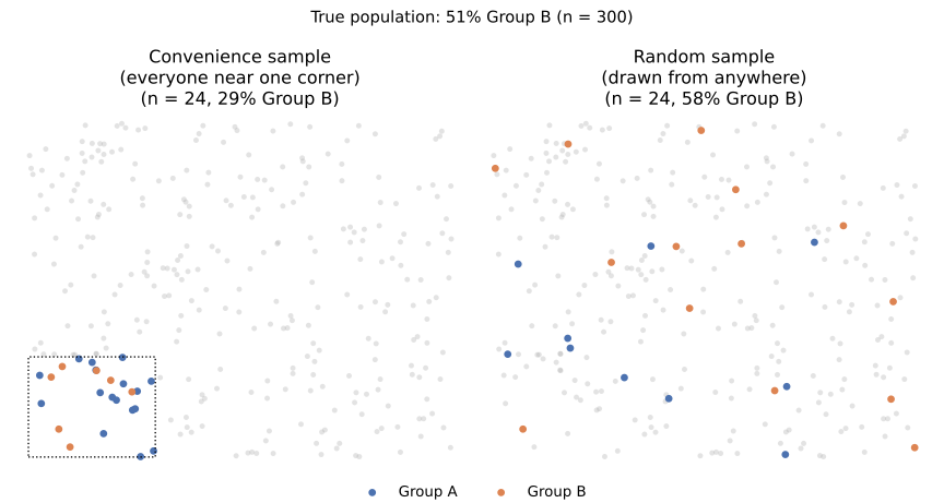
The same simulated population sampled two ways: a spatially clustered convenience sample distorts the mix of the two groups, while a random sample tracks the true population proportions.drawn by figures/fig-biased-vs-random-sample.py

The trap

"Random sampling just means grabbing whoever's around or easy to reach." That's convenience, not randomness: a random method gives every member a known chance, which grabbing whoever's around never does. "If enough people respond, the sample is fine no matter how they were chosen — a large sample can't be biased." More responses collected the same flawed way just repeat the flaw, as the case below shows. "Letting people decide for themselves whether to respond is the fairest, least biased way to build a sample." This is voluntary response: strong opinions respond far more often than everyone else.

Case

In 1936 the Literary Digest, a popular U.S. magazine, mailed roughly ten million presidential-election questionnaires and received about 2.4 million back — a sample far larger than any modern poll uses. It predicted the challenger would win comfortably; the incumbent won in a landslide. The magazine's mailing list came from its own subscribers, automobile registration records and telephone directories, which in 1936 skewed toward wealthier, Depression-insulated households, and only about one in four recipients replied, adding voluntary response on top of undercoverage. Millions of responses did not save a flawed method.

Expanded

What makes a simple random sample simple is stronger than every individual having a fair chance: every possible group of $n$ people is equally likely to be the one chosen. The weaker property on its own does not single out the simple random sample — a systematic sample gives each person a 1-in- $k$ chance too, yet the groups it can produce are only the evenly spaced ones.

Beyond the simple random sample, three standard variations are also random sampling in the technical sense — the method decides who's included, never the individual or the researcher's convenience. A stratified sample divides the population into groups (say, by year of study) and takes a proportionate number from each. A cluster sample divides the population into clusters (say, by dorm building) and randomly selects entire clusters rather than individuals. A systematic sample picks a random starting point, then takes every $k$ -th person from a list. All three are legitimate alternatives to a plain simple random sample, chosen for cost or logistics, not a compromise on fairness.

Bias is also worth separating from two look-alikes. Sampling error is the ordinary difference between a sample and the population that comes from sampling at all rather than measuring everyone — a form of that shrinks, on average, as the sample grows, and is nobody's mistake. Nonsampling error is different again: a mistake unrelated to the sampling process itself, like a mistyped number or a broken scale. Bias is a third thing, distinct from both — a systematic pull in one direction that no amount of additional data, collected the same flawed way, will average out. A larger simple random sample reduces sampling error; no sample size fixes bias, because bias lives in the method, not the count.

Same Population, Different Sample, Different Number

Definition

Sampling variability is the natural difference between computed from different random samples of the same population — expected variation from chance, not .

The test

Two honestly random samples of the same size almost never produce identical statistics, and neither is "wrong." Ask why they differ: different individuals caught by chance is variability; a method that favors some individuals is instead.

Example

Back to the example: the school of 4,000 students. You survey 50 random students and get an average GPA of 3.1; a classmate surveys a different 50 and gets 3.4. Neither of you erred — you simply didn't survey the same people.

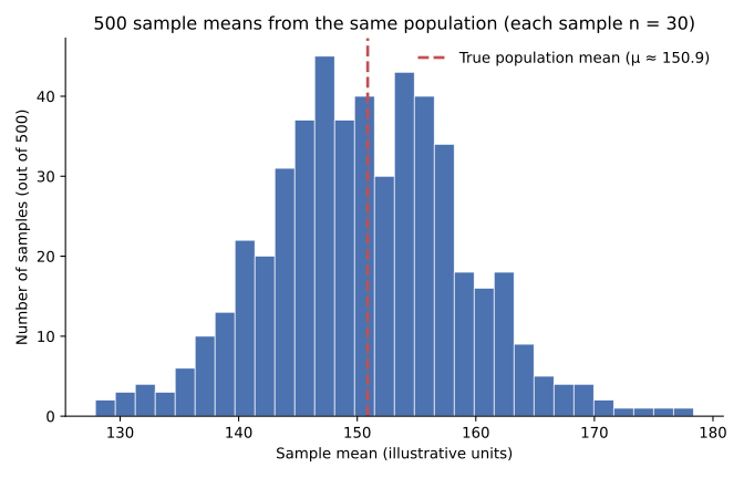
500 sample means from repeated random samples of size 30, drawn from the same simulated population, cluster around the true population mean but rarely land on it exactly.drawn by figures/fig-sampling-variability.pyThis figure becomes interactive in the app.

The trap

"If I repeated the survey with a new sample, I should get the same number as before — a different result means something went wrong." Nothing went wrong: a fair method still varies draw to draw, because who it happens to catch varies by chance — that's what randomness means. "Sampling variability and sampling bias are basically the same problem — both just mean the sample can't be trusted." They aren't: bias comes from how a sample is chosen; variability comes from which members a fair method happened to select, and it survives even after bias is eliminated.

Expanded

What does shrink sampling variability is a larger sample: a properly selected bigger sample tends to land closer to the true parameter $\mu$ on average, and the spread across repeated samples narrows. This is easy to confuse with the bias question, so it is worth stating plainly: a larger sample size shrinks sampling variability, but does nothing to shrink , because bias comes from the method, not the count. This is precisely why serious polls and studies report a margin of error alongside a headline number instead of a bare figure — that margin is an honest, quantified admission that an equally valid random sample of the same size would very likely have landed on a somewhat different statistic. If you and a classmate each took ten more random samples of 50 students, you would not expect all ten of either of your statistics to match each other exactly; you'd expect a spread of similar, not identical, numbers, clustered near the population's true, unknown $\mu$ .

Categorical or Quantitative: What Kind of Data Is It

Definition

Categorical data (also called qualitative data) sorts each individual into a group or label; quantitative data is a count or measurement you can meaningfully do arithmetic on.

The test

Ignore whether a value is written with digits or words. Ask whether adding or averaging two values produces an answer that means anything. If yes, quantitative. If no, categorical.

Example

A class roster lists a student's hair color as "brown" and student ID as "10583." Hair color is categorical. The ID, despite being all digits, is categorical too: averaging two IDs, or calling one "greater than" another, means nothing — it's a label wearing a costume of digits.

The trap

"If it's written down as a number, it's quantitative; if it's written as words, it's categorical." ZIP codes, phone numbers, and jersey numbers are all-digit and still categorical, by the arithmetic test above. "Categorical data can't really be analyzed with numbers, only described in words." You can count how many individuals fall into each category and compare those counts or proportions — what you can't do is average the categories themselves, because "brown" plus "blond" divided by two is not a hair color.

Counting or Measuring: Discrete and Continuous Data

Definition

Discrete data comes from counting and takes separate, listable values with real gaps between them; continuous data comes from measuring and can fall anywhere on a scale.

The test

Ask whether a value strictly between two consecutive data points is possible even in principle. If yes, continuous. If no, discrete. Decimals aren't the test: a discrete count can average out to a decimal, and a continuous measurement can land on a whole number.

Example

For a hypothetical class of 30 students, number of siblings and height in centimeters are both . Siblings comes from counting: nothing valid sits between 2 and 3, so it's discrete. Height comes from measuring: a value can land anywhere between 162 and 163 cm, so it's continuous.

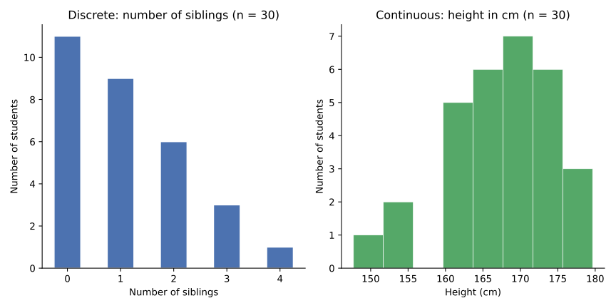
A discrete count (siblings, left) leaves real gaps between the bars; a continuous measurement (height, right) does not.drawn by figures/fig-discrete-vs-continuous.py

The trap

"If the numbers have decimals, the data is continuous; if they're whole numbers, it's discrete." A discrete count can average to a decimal — "the average student has 1.8 siblings" is normal, even though no student has 1.8 siblings; the decimal belongs to the average, not any single count. "Continuous just means there are a lot of different values in the data." A continuous measurement can also land exactly on a whole number by coincidence, like a student genuinely 170.0 cm tall — what matters is whether in-between values are possible.

Putting the Pieces TogetherSynthesis

One last hypothetical: a college wants to know whether its students prefer online or in-person classes — the split again, the whole student body versus whoever you actually collect.

Standing in the quad and asking whoever walks by is a problem called undercoverage: students who aren't there at that hour get no chance. Posting the survey online and taking all comers has the opposite bias, voluntary response, overrepresenting strong feelings. What you want instead is closer to a simple random sample, giving every student a known, fair chance.

Whatever sample you get, the share who prefer online classes is a statistic — your best evidence about the true , the actual share across the whole college, never known exactly. A classmate's equally valid survey landing on a slightly different number would be ordinary , not a mistake.

Along the way: a student's preference is ; how many online classes they've taken is quantitative and discrete; weekly commute hours are quantitative and . None of these six is optional — each is a way a confident number can mislead you if you don't ask what kind it is.

Sources

1 OpenStax Introductory Statistics §1.1: Definitions of Statistics, Probability, and Key Terms — source
2 OpenStax Introductory Statistics §1.2: Data, Sampling, and Variation in Data and Sampling — source
3 The Literary Digest 1936 presidential poll — source